Computers and humans process language very differently. For humans, words combine to form meaningful sentences that convey information. However, for computers, sentences are simply collections of words, or tokens, that only make sense in relation to other documents. This difference can make information retrieval systems less effective, as two phrases with the same meaning might go unrecognized by a computer if they don’t contain similar words. This is a limitation of keyword-based search systems, like when you use ‘ctrl+f’ on a webpage to find an exact phrase. More advanced systems can break down your input into words and return sentences that contain most or all of those words, even if they’re not in the same order. Some systems go further by removing common words (stopwords) or grouping similar words (stemming) to focus more on the intent of your search.
Recent advancements in natural language processing (NLP) have given us language models that can understand the meaning behind words and sentences, converting them into numerical representations (vectors) using machine learning. In our project, we explore how this can be applied to Twitter, where tweets are short (up to 280 characters) and users only interact with them briefly. Traditional keyword searches can struggle with such small pieces of text, and users often don’t remember the exact wording when trying to find a tweet. This is why we wanted to explore vector search as a better alternative.
System Design
The domain model diagram we created outlines the components of our system. We started with a Twitter dataset containing random tweets from various users. Although the dataset also included images, adding them increased the size from under 10GB to over 40GB, so we chose to exclude them. For embedding the text data, we used Google’s BERT multi-qa-MiniLM-L6-cos-v1 pretrained model, which trades a bit of accuracy for faster embedding.
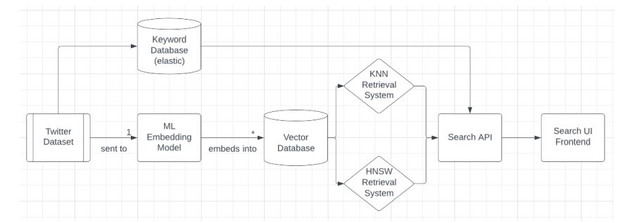
We indexed the embedded vectors into a database and retrieval system. Although we considered using Pinecone for its “vector search as a service” feature, we opted to host our indices using FAISS (Facebook AI Similarity Search). FAISS offers both KNN and HNSW indexing, allowing us to build and compare both methods. We also created a local elastic cluster using Docker to handle the raw tweets, as elastic doesn’t require embeddings. The search API, built with Flask, connects with the TypeScript and Vue front end through post requests to manage the queries.
Product Functionality
Our product has certain capabilities and limitations that are important to understand. It doesn’t replace Twitter’s original search system, and currently, it can’t search for images based on their descriptions. However, with more resources and adjustments, we could update the system to support this by using a different embedding model for images. The only changes needed would be how images are stored (since they can’t go into a CSV) and a slight increase in the time it takes to search the database. Despite these limitations, our product delivers most of the key features we aimed for. It efficiently converts text into vectors, allowing us to manage large amounts of data.
The system stores these embeddings and indices in memory, which makes it quick to start and stop. Users can easily interact with the database through a user-friendly interface, and the product supports comparison between three different data retrieval methods, showing both the results and the time it took to retrieve them.
How to use the product
On Twitter, using our dataset would be a trivial process for end users since they would interact with it through the same search bar exactly as they have always done. The only difference would be on the backend and, hopefully, in the improved results that they see. For Twitter engineers, the process would change more significantly, but the net result is still using a service to query a database to find results.
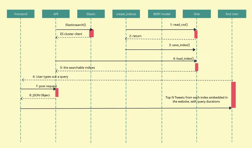
As-is, our system works differently. In order to run it from start to finish, you would first need to find a dataset, run our embedding script, run our create_indices script, and create the elasticsearch docker container using the new dataset, all of which needs to be done only once. After those are completed, spinning up the indices is as simple as running the docker container, starting the frontend using npm, and using Anaconda to run the API flask app. Once there, the process is quite simple and mostly handled on the backend.
The development process
We’ve already talked about the design of the system, so let’s talk briefly about the development.
1. Preprocessing
Preprocessing is traditionally a large part of any NLP project, especially for Twitter data. Interestingly, BERT’s sentence transformer models are trained on near raw data for the most part, which means that the rigorous preprocessing steps of stemming, lemmatization, stopword removal, etc., were not necessary for our project. As a result, the preprocessing that we did was essentially just removing retweets from our dataset.
2. Embeddings
Creating the embeddings was a challenging process for us. Initially, we researched different types of embeddings and found that while Word2Vec is a popular ‘last-generation’ method, sentence transformers are more effective but less documented due to their cutting-edge nature. We decided to use Google’s BERT pretrained models, which suited our needs well. These models range from single-language to multilingual and even multimodal, covering various levels of accuracy and efficiency. For our project, we chose an English text-only model optimized for efficiency due to the computational demands of other models and the data they would require.
Each model takes a string as input and outputs a 1xD vector, where D varies by model. In our case, the model produced 384-dimensional vectors. The embedding process itself was straightforward since we used pretrained models. We just had to install the module, load it into our script, initialize it with the chosen model key, and then use `model.encode()` on each document. The challenge, however, was handling and storing a large amount of data. We had 3.4 million records, and even though encoding each document took only a fraction of a second, the entire process took dozens of hours. Fortunately, we were able to speed this up using GPU acceleration, making it ten times more efficient.
The real difficulty was efficiently storing the embeddings. We needed to maintain the connection between the 1×384 vector and the original text document. Our first thought was to store them in a pandas data frame, but pandas didn’t support this well. We tried two approaches: serializing and deserializing the arrays, which led to issues with interpreting the byte stream as a string, and overriding the pandas column dtype to an object, which forced us to use a for loop, drastically slowing down our code. Eventually, we solved this by linking the embeddings and documents in different files using a common index. However, this introduced a new problem—out-of-memory (OOM) issues when processing the entire document dataset at once. To handle this, we used `pd.read_csv` with the `chunksize` argument to process the data in smaller batches and write the results incrementally. Since `nparray.save` doesn’t support piecewise appending, we had to use two different file-handling modes: the documents were processed in chunks, embedded, and saved to a new file, while the embedding array was stored in memory and written at the end. This approach worked because the embeddings only took up about 4.5GB, which was manageable when not storing the full document dataset in memory simultaneously.
3. FAISS indices
Surprisingly, the process of populating the FAISS indices and querying them was one of the easier aspects of our project. The library documentation is quite bad and ironically unsearchable for some reason, but there are enough resources out there that once you understand what to do, it’s only a few function calls away. FAISS supports both flatIndexL2 and flatHNSWIndex, which makes our job easier since we don’t have to implement HNSWs ourselves. We could have optimized our indices using a variety of methods that they support, but we left that for future work.
4. Elastic
The elastic search component uses the elastic/elasticsearch GitHub repo solution. This is an open-source solution that works through a docker container from which you can index and get data from. The data is built using a script that sends HTTP requests to the docker container, which indexes all the tweets. Afterwards, the data can be requested by pinging the /search endpoint in the backend API. This sends a request to find any content with a given keyword in the elastic search container.
5. Frontend
The frontend was coded using the Vue.js frontend framework, which consisted of Vue.js, Typescript, HTML, and CSS. Given the fact that the functionality of this project was essentially a proof of concept/test of the different search systems, we did not spend much time designing the front end; instead, we chose to focus primarily on the back end. As a result, the front end was the final thing to be completed. This was also partially because we all had limited front-end experience.
6. Testing / Results
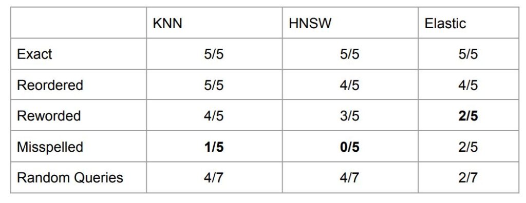
For testing our project we decided to take 5 tweets out of our dataset, permute them in various ways, and count the successful recalls of the different systems, then create 7 random queries and qualitatively judge the results based on relevance. The results that we got are below:
We measured the retrieval times for KNN, HNSW, and Elastic search and plotted the results. The average times were 0.3885 seconds for KNN, 0.1752 seconds for HNSW, and 0.1036 seconds for Elastic. This shows that Elastic was the fastest on a smaller dataset, though HNSW was significantly quicker than KNN. HNSW even outperformed Elastic at times, whereas KNN was always slower.
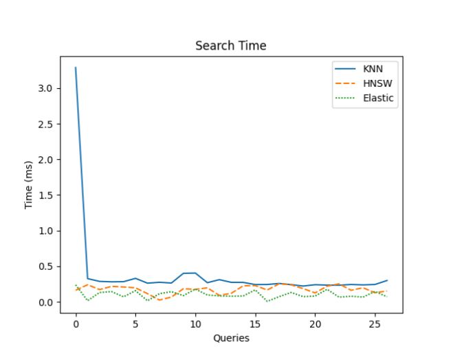
In terms of recall, KNN was the most accurate, except for misspelled queries. Both vector-based methods (HNSW and Elastic) performed better with random and reworded queries. These results make sense since our FAISS indices used raw data and couldn’t process unknown words. Elastic, however, has features like hamming score and basic autocorrect, helping it handle misspelled queries better. However, Elastic struggled with heavily reworded queries (changing 75-100% of the words), where it often failed to find the correct document, but FAISS succeeded more often. The one surprise was that FAISS outperformed on random queries, which we didn’t fully expect but were pleased to see.
7. Retrospective
There were a lot of things that went really well for us during this project. We were able to quickly learn most of the technical elements that we needed to work with throughout this project, including machine learning, API development, frontend design, web app development, and dockerizing the elasticsearch cluster. We set our hopes quite high with the scale and complexity of the systems we wanted to make, but we were able to accomplish it all in this limited time frame. One thing that we talked about taking to other projects that we will work on in the future is the software that we use to make sure that information is always available to every member of the team. We updated each other constantly in our group chat, we kept the code up to date in the GitLab repository, our drive contained all relevant files that any of us would need to use, and when researching and designing our system early in the semester, we used a Notion page to be able to store all of the links and information that we had gathered. It takes a lot of active work to keep communication that good, but for the most part, we’re proud of how we kept each other up to date. As far as things that didn’t go as well, consistency is probably the easiest answer. We had several weeks where we accomplished a lot and several weeks where little to nothing got done. If we had put in 70% effort every week instead of 100% every 2 or 3 weeks, we probably would have been able to get a lot more of our reach objectives completed and been able to finish mistakes that we would have realized earlier on in the project. We also didn’t keep our dataset consistent between the two index tracks, which hurts the validity of our data. We talked about communication being a really important part, but something that we didn’t really communicate was the internal logic of each individual component. Sometimes, we would brief each other on the basics, but going in-depth enough to understand things like the cleaning methods of the dataset wasn’t something that we did. In retrospect, we should have had the foresight to clean the dataset and then split the work instead of getting the dataset, splitting the job, and then preprocessing it individually.


