Introduction
In various data-driven fields such as data science, similarity search frequently arises within the realm of natural language processing (NLP), search engines, and recommender systems, tasked with identifying the most pertinent documents or items related to a given query. Enhancing search efficiency in vast datasets encompasses a diverse array of methodologies.
Hierarchical Navigable Small World (HNSW) stands out as a cutting-edge algorithm employed for approximating nearest neighbour searches. Leveraging optimized graph structures, HNSW operates distinctively from conventional methods, rendering it a formidable tool in the realm of similarity search.

Before delving into the intricacies of HNSW, it’s essential to explore skip lists and navigable small worlds, pivotal data structures employed within the HNSW framework.
Skip lists
Skip list, a probabilistic data structure, facilitates efficient insertion and search operations within a sorted list, boasting an average complexity of O(logn). This structure comprises multiple layers of linked lists. At its base lies the original linked list containing all elements. As one ascends through the layers, the number of elements skipped grows, resulting in fewer connections and expedited traversal.
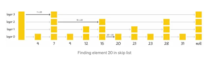
The search procedure for a particular value commences at the highest level, where it evaluates the next element against the sought-after value. If the value is either less than or equal to the element, the algorithm advances to the subsequent element. Conversely, if the value surpasses the element, the search procedure transitions to a lower layer characterized by more extensive connections, repeating the comparison process. Ultimately, the algorithm descends to the lowest layer to pinpoint the desired node.
Drawing from insights on Wikipedia, skip lists introduce a pivotal parameter denoted as p, which determines the likelihood of an element appearing in multiple lists. If an element is present in layer i, the probability of its presence in layer i + 1 equals p (typically set to 0.5 or 0.25). On average, each element manifests in approximately 1 / (1 — p) lists.
Evidently, this approach outpaces the conventional linear search method employed in linked lists. Notably, HNSW adopts a similar concept, albeit utilizing graphs instead of linked lists.
Navigable Small World
Navigable Small World graph is characterized by its polylogarithmic search complexity, denoted as T = O(logᵏn), wherein the process of greedy routing is employed. Routing in this context involves initiating the search from vertices with low degrees and progressing towards those with higher degrees. This strategic approach leverages the sparse connections of low-degree vertices to swiftly traverse between them, facilitating efficient navigation towards the area where the nearest neighbor is anticipated to reside. Subsequently, the algorithm seamlessly transitions to high-degree vertices, gradually narrowing down the search space to pinpoint the nearest neighbor within that specific region.
| Vertex is sometimes also referred to as a node. |
Search
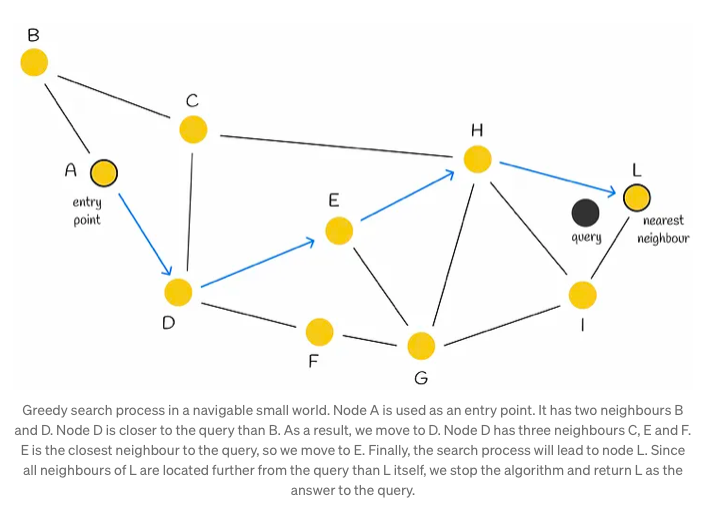
Initially, the search process commences with the selection of an entry point. This pivotal step sets the stage for subsequent vertex determinations within the algorithm. The next vertex, or vertices, are determined based on the calculation of distances from the query vector to the neighboring vertices of the current vertex. Subsequently, the algorithm progresses by moving towards the closest vertex. Eventually, the search reaches its conclusion when there are no neighboring nodes closer to the query than the current node, which is then returned as the query’s response.
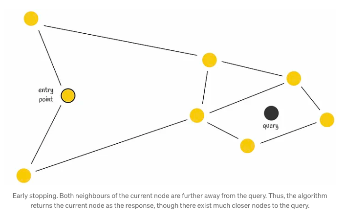
Although employing a greedy strategy, this approach lacks a guarantee of finding the precise nearest neighbor, relying solely on local information at each step to dictate its decisions. Notably, a common issue encountered is early stopping, particularly noticeable at the outset of the search process, where superior neighboring nodes are absent. This predicament is exacerbated in scenarios with an abundance of low-degree vertices within the starting region.
To enhance search accuracy, employing multiple entry points proves advantageous.
Construction
The construction process of the NSW (Neighborhood Subgraph Walk) graph involves iteratively incorporating dataset points into the existing graph through shuffling and sequential insertion. Upon insertion of a new node, it establishes connections with the M nearest vertices, fostering the formation of edges that facilitate efficient graph navigation.
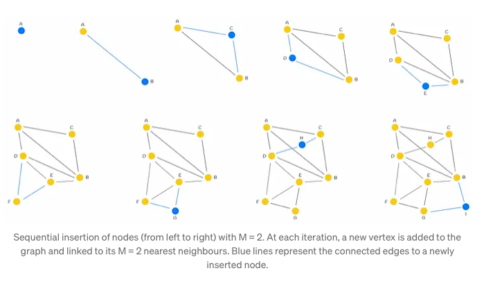
Typically, during the initial stages of graph construction, longer-range edges tend to emerge, serving as pivotal conduits for traversing the graph. These edges assume significance in enabling seamless navigation throughout the network.
Illustrated in the accompanying figure is the significance of an early-introduced long-range edge, exemplified by AB. This edge, forged in the initial stages, proves invaluable for scenarios requiring traversal between distant nodes such as A and I. By bridging disparate regions of the graph, the AB edge facilitates swift navigation, enhancing query efficiency.
Furthermore, as the graph expands with the addition of more vertices, there arises an augmented likelihood of shorter lengths for newly established edges connecting to a freshly incorporated node. This phenomenon contributes to the continual refinement and densification of the graph structure, fostering enhanced connectivity and traversal efficiency.
HNSW
HNSW, or Hierarchical Navigable Small World, operates on foundational principles akin to those found in skip lists and navigable small worlds. This innovative approach entails a multi-layered graph structure, where the upper layers exhibit sparser connections while the lower layers comprise denser regions. This hierarchical arrangement enables efficient navigation and proximity searches within the data space, facilitating quicker retrieval of relevant information.
Search
The search process begins at the uppermost layer and systematically descends, iteratively identifying the nearest neighbor within each layer’s node set. This methodically progresses until the closest neighbor within the lowest layer is determined, serving as the final answer to the query at hand.
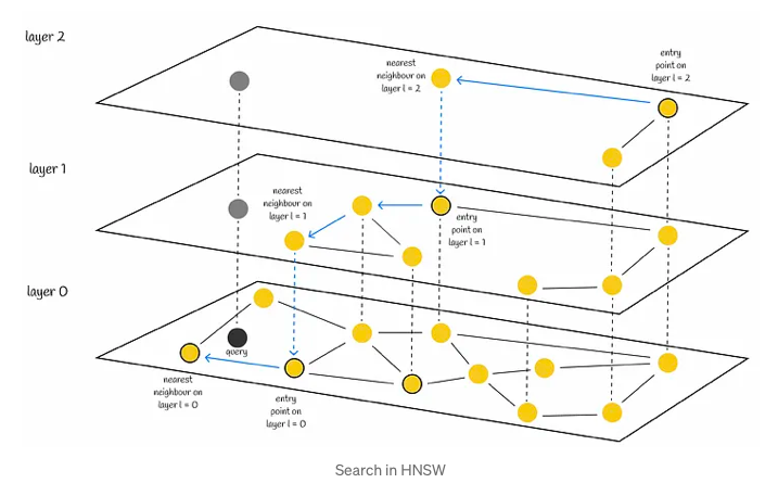
In a manner akin to NSW, the efficacy of HNSW’s search can be heightened through the utilization of multiple entry points. Rather than solely identifying a single nearest neighbor within each layer, the process of efSearch, governed by a hyperparameter, locates a specified number of closest nearest neighbors to the query vector. Subsequently, each of these neighbors serves as an entry point for the subsequent layer, enhancing the overall search quality.
Complexity
The original paper’s authors assert that the computational effort needed to locate the nearest neighbor at any layer remains within a constant limit. This assertion holds true when considering that the quantity of layers within a graph follows a logarithmic progression. Consequently, the cumulative search complexity can be described as O(logn), where ‘n’ represents the total number of layers in the graph.
Construction
Choosing the maximum layer
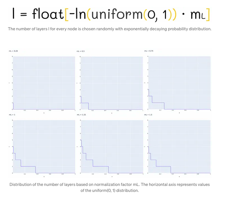
In the Hierarchical Navigable Small World (HNSW) structure, nodes are incrementally inserted one by one. Each node undergoes a random assignment of an integer parameter, denoted as ‘l’, which signifies the maximum layer it can occupy within the graph. For instance, if ‘l’ equals 1, the node is confined to layers 0 and 1. The determination of ‘l’ for each node follows an exponentially decaying probability distribution, a process normalized by the non-zero multiplier mL. Setting mL to 0 confines nodes to a single layer, thus leading to suboptimal search complexity in HNSW. Typically, a majority of ‘l’ values tend to be 0, resulting in most nodes residing solely on the lowest level. However, higher values of mL elevate the likelihood of nodes being positioned on upper layers, potentially enhancing the structure’s efficiency.
One strategy for mitigating overlap involves reducing the parameter mL. However, it’s crucial to note that diminishing mL concurrently results in an increase in traversals during a greedy search across layers, on average. Hence, striking a balance between overlap reduction and traversal count is paramount. The authors advocate for selecting an optimal mL value, specifically suggested as 1 / ln(M), where M represents a parameter in the skip list. This choice aligns with achieving an average single-element overlap between layers, denoted by the parameter p = 1 / M.
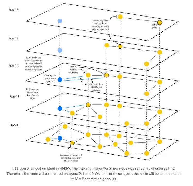
Insertion
Upon assignment of the value l to a node, the insertion process unfolds in two distinct phases:
- Firstly, the algorithm initiates from the upper layer, meticulously seeking out the closest node. This node then serves as the gateway to the subsequent layer, perpetuating the search process. Upon reaching layer l, the insertion advances to the second phase.
- In the second phase, commencing from layer l, the algorithm embeds the new node within the current layer. It mirrors the preceding step, but instead of identifying a single nearest neighbor, it expansively seeks efConstruction (hyperparameter) nearest neighbors. Subsequently, M out of these efConstruction neighbors are selectively chosen, and connections are established from the inserted node to them. Following this, the algorithm progresses downward to the next layer, where each of the identified efConstruction nodes acts as an entry point. The culmination of the algorithm occurs once the new node and its corresponding edges are integrated into the lowest layer, layer 0.
Choosing values for construction parameters
The original paper offers valuable insights into the selection of hyperparameters, elucidating optimal choices through simulations. These simulations suggest that for parameter M, a range between 5 and 48 yields favorable results. Lower values of M demonstrate efficacy in scenarios with lower recalls or lower-dimensional data sets, whereas higher values are more adept at handling high recalls or high-dimensional data.
The parameter efConstruction, denoting the intensity of search exploration, plays a pivotal role. A higher efConstruction value facilitates a deeper search by exploring more candidates but demands increased computational resources. The authors advocate for selecting an efConstruction value that maintains recall levels close to 0.95–1 during training, striking a balance between thorough exploration and computational efficiency.
Furthermore, there’s significance attached to Mₘₐₓ, representing the maximum number of edges per vertex, and Mₘₐₓ₀, specifically for the lowest layer. It’s advised to set Mₘₐₓ around 2 times M, as values exceeding this threshold may result in performance deterioration and excessive memory usage. Conversely, setting Mₘₐₓ equal to M can compromise performance at higher recall levels. Thus, careful consideration of these parameters is crucial for optimal model performance.
Candidate selection heuristic
In the process of node insertion, a selection is made from a pool of efConstruction candidates, with M nodes being chosen to establish edges. Delving into the methodology of selecting these M nodes, various approaches can be explored to optimize the outcome.
One straightforward method involves selecting the M closest candidates. However, this simplistic strategy may not consistently yield the most advantageous results, as illustrated by the following example.
Consider a graph depicted in the accompanying figure, characterized by its distinct regions, some of which are disconnected from each other (notably, the left and top regions). Traversing from point A to B necessitates a circuitous route through another region due to this lack of connectivity. In such scenarios, there arises a logical imperative to establish connections between these isolated regions to facilitate more efficient navigation and pathfinding.
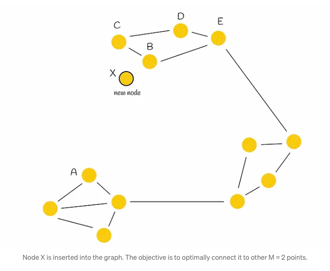
In the given scenario, when a new node X is introduced into the graph and requires connections to M = 2 other vertices, the conventional method would simply link X to its M = 2 closest neighbors (designated as B and C). However, while this establishes connections with immediate neighbors, it fails to fully address the underlying issue at hand. To tackle this, the authors propose a heuristic approach, which we shall delve into for a more nuanced understanding.
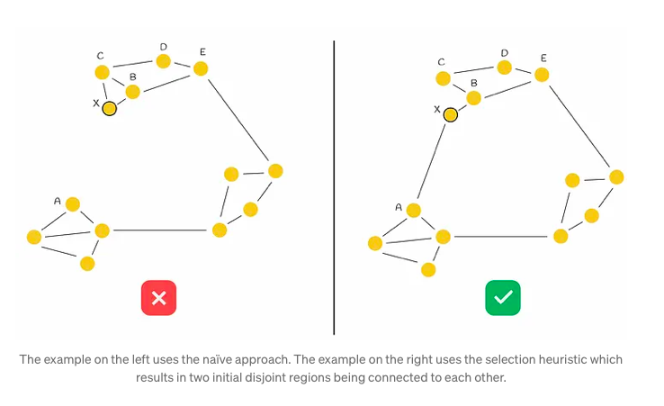
The heuristic algorithm initiates by selecting the nearest neighbor (denoted as B in our scenario) and establishing a connection between the newly inserted node (referred to as X) and B. Subsequently, it iteratively identifies the next closest neighbor in a sorted sequence (designated as C), only forming an edge with it if the distance from this neighbor to the new node X is shorter than any distance from the neighbor to all previously connected vertices (B) to X. This iterative process continues until M edges have been established.
Illustrating this process with an example, the heuristic initially selects B as the closest nearest neighbor to X and creates the edge BX. The subsequent selection of C as the next closest neighbor reveals that BC < CX, indicating that adding the edge CX to the graph is suboptimal due to the proximity of nodes B and C and the preexistence of edge BX. This evaluation extends similarly to nodes D and E. The algorithm then assesses node A, where it satisfies the condition BA > AX, consequently forming the new edge AX and establishing connectivity between both initial regions. This step-by-step process is depicted in the accompanying figure below.
Complexity
The insertion process closely mirrors the search procedure, exhibiting no substantial distinctions that would necessitate a variable number of operations. Consequently, the insertion of each individual vertex demands O(logn) time. To gauge the overall complexity, one must take into account the total number of inserted nodes, denoted as n, within the dataset. Consequently, the construction of an HNSW structure mandates O(n * logn) time.
Combining HNSW with other methods
HNSW can significantly enhance performance when employed in conjunction with other similarity search techniques. One highly effective approach involves integrating HNSW with an inverted file index and product quantization (IndexIVFPQ), as detailed elsewhere in this series.
In this context, HNSW serves as a crucial component, acting as a coarse quantizer for IndexIVFPQ. Its primary function is to locate the nearest Voronoi partition, thereby reducing the search scope. This process entails constructing an HNSW index on all Voronoi centroids. When presented with a query, HNSW is utilized to identify the nearest Voronoi centroid, replacing the previously employed brute-force search method which involved comparing distances to every centroid. Subsequently, the query vector undergoes quantization within the relevant Voronoi partition, and distances are computed using PQ codes.
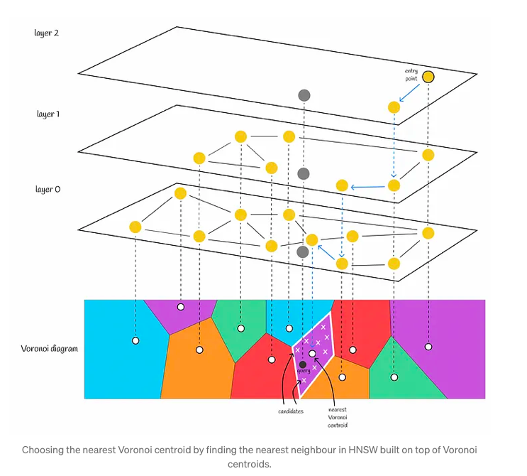
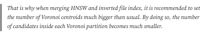
When utilizing solely an inverted file index, it is advisable to limit the number of Voronoi partitions to a moderate size, such as 256 or 1024. This is due to the fact that a brute-force search is employed to locate the nearest centroids. Opting for a smaller number of Voronoi partitions results in a relatively larger number of candidates within each partition. Consequently, the algorithm swiftly discerns the nearest centroid for a query, with the majority of its computational effort focused on identifying the nearest neighbor within a Voronoi partition.
However, the integration of HNSW into the workflow necessitates a strategic adjustment. Implementing HNSW solely on a limited set of centroids, such as 256 or 1024, may not yield significant benefits. This is because, with a restricted number of vectors, HNSW’s execution time is comparable to that of naïve brute-force search. Furthermore, employing HNSW would entail a higher memory overhead for storing the graph structure.
This fundamental shift in paradigm yields significant outcomes within the following settings:
- HNSW, leveraging its efficient algorithm, swiftly pinpoints the nearest Voronoi centroids with remarkable speed, operating within logarithmic time complexity.
- Subsequently, a meticulous exploration ensues within the designated Voronoi partitions. This task is facilitated by the inherently limited number of potential candidates, minimizing computational burden and ensuring streamlined processing.
Faiss implementation
Faiss, short for Facebook AI Search Similarity, emerges as a highly efficient Python library primarily crafted in C++, purpose-built to facilitate optimized similarity search tasks. Renowned for its prowess, this library introduces a diverse array of indexes, sophisticated data structures meticulously designed to not only store data effectively but also execute queries with remarkable efficiency.
Delving into the depths of Faiss documentation, we embark on a journey to explore the utilization and amalgamation of HNSW, an algorithmic gem, seamlessly blending it with the prowess of inverted file index and product quantization.
IndexHNSWFlat
FAISS has a class IndexHNSWFlat implementing the HNSW structure. As usual, the suffix “Flat” indicates that dataset vectors are fully stored in index. The constructor accepts 2 parameters:
- d: data dimensionality.
- M: the number of edges that need to be added to every new node during insertion.
Additionally, via the hnsw field, IndexHNSWFlat provides several useful attributes (which can be modified) and methods:
- hnsw.efConstruction: number of nearest neighbors to explore during construction.
- hnsw.efSearch: number of nearest neighbors to explore during search.
- hnsw.max_level: returns the maximum layer.
- hnsw.entry_point: returns the entry point.
- faiss.vector_to_array(index.hnsw.levels): returns a list of maximum layers for each vector
- hnsw.set_default_probas(M: int, level_mult: float): allows setting M and mL values respectively. By default, level_mult is set to 1 / ln(M).
| d = 256
M = 32 index = faiss.IndexHNSWFlat(d,M) index.hnsw.efConstruction = 64 index.hnsw.efSearch = 32 index.set_default_probas(32, 0.4) index.add(data) print(f”Maximum layer : {index.hnsw.max_level}”) print(f”Entry point : {index.hnsw.entry_point}”) Levels = faiss.vector_to_array(index.hnsw.levels) print(f”Maximum layer for each vector: {levels}”) print(f”Distribution of levels: {np.bincount(levels)}”) k = 3 D, I = index.search(query, k) |
IndexHNSWFlat sets values for Mₘₐₓ = M and Mₘₐₓ₀ = 2 * M
IndexHNSWFlat + IndexIVFPQ
IndexHNSWFlat can be combined with other indexes as well. One of the examples is IndexIVFPQ described in the previous part. Creation of this composite index proceeds in two steps:
- IndexHNSWFlat is initialized as a coarse quantizer.
- The quantizer is passed as a parameter to the constructor of IndexIVFPQ.
Training and adding can be done by using different or the same data.
| d = 256
M = 64 nlist = 8192 nsubspace = 32 nbits = 8 quantizer = faiss.IndexHNSWFlat(d,M) Index = faiss.IndexIVFPQ(quantizer, d, nlist, nsubspace, nbits) index.train(data) index.add(data) Index.nprobe = 10 k = 3 D, I = index.search(query, k) |